Types of ML

Types of ML#

Supervised Learning#

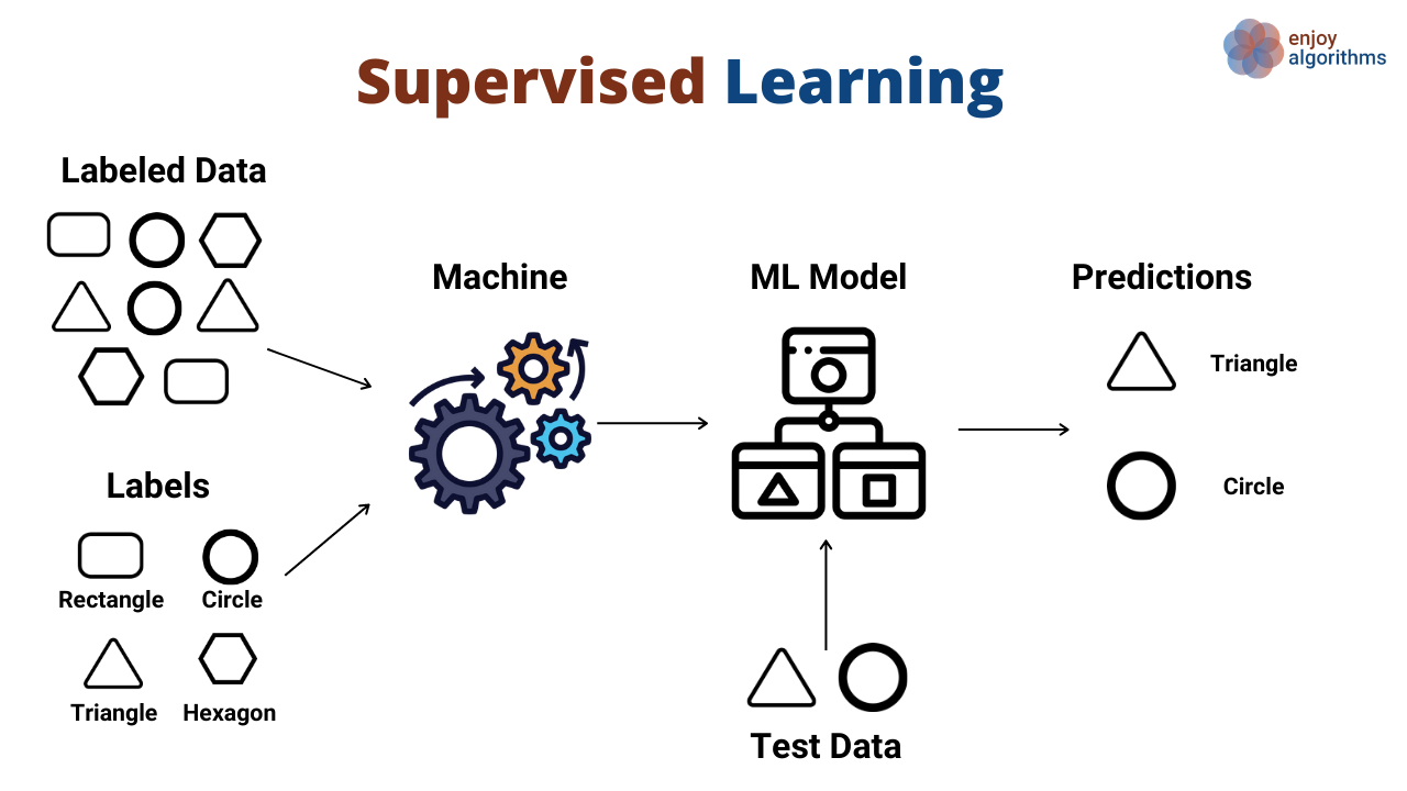
Supervised learning is a popular category of machine learning algorithms that involves training a model on labeled data to make predictions or decisions. In this approach, the algorithm learns from a given set of input-output pairs and uses this knowledge to predict the output for new, unseen inputs. The goal is to find a mapping function that generalizes well to unseen data.

Now put it more mathematically. Denote

training dataset \(\mathcal D = \{(\boldsymbol x_i, y_i)\}_{i=1}^N\);
features \(\boldsymbol x \in \mathcal X\) (usually \(\mathcal X = \mathbb R^D\));
targets (labels) \(y_i \in \mathcal Y\).

The goal of the supervised learning is to find a mapping \(f\colon \mathcal X \to \mathcal Y\) which would minimize the cost (loss) function

\[ \mathcal L = \frac 1N \sum\limits_{i=1}^N \ell(y_i, f(\boldsymbol x_i)). \]

Note that the loss \(\ell(y_i, f(\boldsymbol x_i))\) is calculated separately on each training object \((\boldsymbol x_i, y_i)\), and then averaged over the whole training dataset.

Predictive model#

The mapping \(f_{\boldsymbol \theta}\colon \mathcal X \to \mathcal Y\) is usually taken from some parametric family

\[ \mathcal F = \{f_{\boldsymbol \theta}(\boldsymbol x) \vert \boldsymbol \theta \in \mathbb R^n\} \]

which is also called a model.

To fit a model means to find \(\boldsymbol \theta\) which minimizes the loss function

\[ \mathcal L(\boldsymbol \theta) = \frac 1N \sum\limits_{i=1}^N \ell(y_i, f_{\boldsymbol \theta}(\boldsymbol x_i)) \]

Classification#

Binary classification

\(\mathcal Y = \{0, 1\}\) or \(\mathcal Y = \{-1, +1\}\)
denote model predictions as \(\hat y_i = f_{\boldsymbol \theta}(\boldsymbol x_i)\)
typical loss function is misclassification rate

(1)#\[ \mathcal L(\boldsymbol \theta) = \frac 1N \sum\limits_{i=1}^N \big[y_i \ne \hat y_i\big]\]

(it actually equals one minus accuracy)
this loss is not a smooth function, that’s why they often predict which is treated as probability of class \(1\), and then use cross-entropy loss

(2)#\[ \mathcal L(\boldsymbol \theta) = -\frac 1N \sum\limits_{i=1}^N \big(y_i \log(\hat y_i) + (1-y_i) \log(1 - \hat y_i)\big)\]

Important

The value \(0\log 0 = 0\) by definition

Example

Suppose that true labels \(y\) and predictions \(\hat y\) are as follows:

Table 1 Binary classificaton#
\(y\)	\(\hat y\)
\(0\)	\(0\)
\(0\)	\(1\)
\(1\)	\(0\)
\(1\)	\(1\)
\(0\)	\(0\)

Calculate the missclassification rate and cross-entropy loss.

To avoid such problems with loss (2) models usually predict numbers from \((0, 1)\), which are interpreted as probabilities of class \(1\).

Multiclass classification

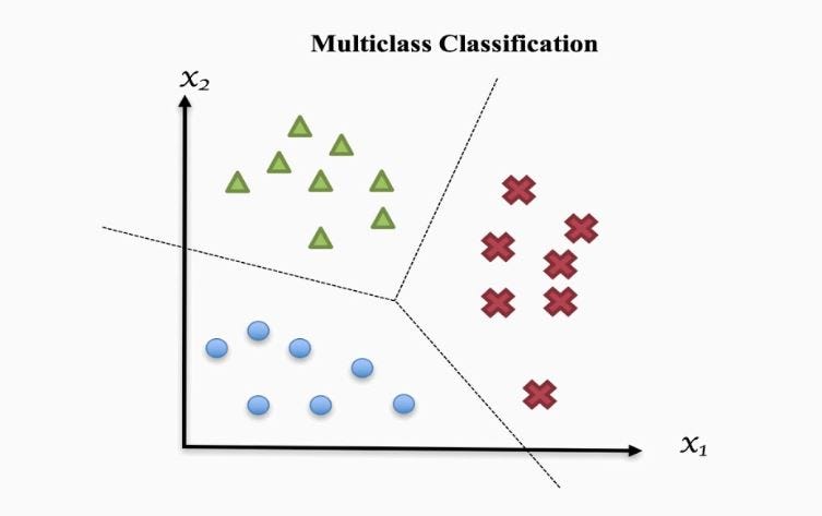
\(\mathcal Y = \{1, 2, \ldots, K\}\)
one-hot encoding: \(\boldsymbol y_i \in \{0, 1\}^K\), \(\sum\limits_{k=1}^K y_{ik} = 1\)
\(\hat{\boldsymbol y}_i = f_{\boldsymbol \theta}(\boldsymbol x_i) \in [0, 1]^K\) is now the vector of probabilities of belonging to class \(k\):

\[ \hat y_{ik} = \mathbb P(\boldsymbol x_i \in \text{ class }k) \]
the cross-entropy loss is now written as follows:

(3)#\[\mathcal L(\boldsymbol \theta) = -\frac 1N \sum\limits_{i=1}^N \sum\limits_{k=1}^Ky_{ik} \log(\hat y_{ik})\]

Example

Classifying into \(3\) classes, model produces the following outputs:

\(y\)	\(\boldsymbol {\hat y}\)
\(0\)	\((0.25, 0.4, 0.35)\)
\(0\)	\((0.5, 0.3, 0.2)\)
\(1\)	\(\big(\frac 12 - \frac 1{2\sqrt 2}, \frac 1{\sqrt 2}, \frac 12 - \frac 1{2\sqrt 2}\big)\)
\(2\)	\((0, 0, 1)\)

Calculate the cross-entropy loss (3). Assume that log base is \(2\).

Regression#

\(\mathcal Y = \mathbb R\) or \(\mathcal Y = \mathbb R^n\)
the common choice is the quadratic loss

\[ \ell_2(y, \hat y) = (y - \hat y)^2 \]
then the overall loss function — mean squared error:

\[ \mathcal L(\boldsymbol \theta) = \mathrm{MSE}(\boldsymbol \theta) = \frac 1N\sum\limits_{i=1}^N (y_i - f_{\boldsymbol \theta}(\boldsymbol x_i))^2 \]

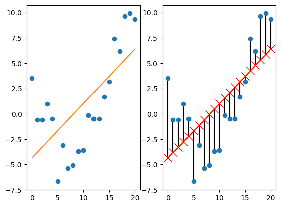
If the function \(f_{\boldsymbol \theta}(\boldsymbol x_i) = \boldsymbol {\theta^\top x}_i + b\) is linear, then the model is called linear regression.

Example of one-dimensional linear regression (figure 1.5 from [Murphy, 2022]):

../_images/96b3dfa5b5dcd31d2d8df9e8c101f08d9868ad8b1c0cf1e6bc2cf381210c1dbf.png

Q. Suppose that training dataset has only one sample (\(N=1\)) and one feature (\(n=1\)). How would linear regression look like in this case? What if \(N=2\)?

Unsupervised learning#

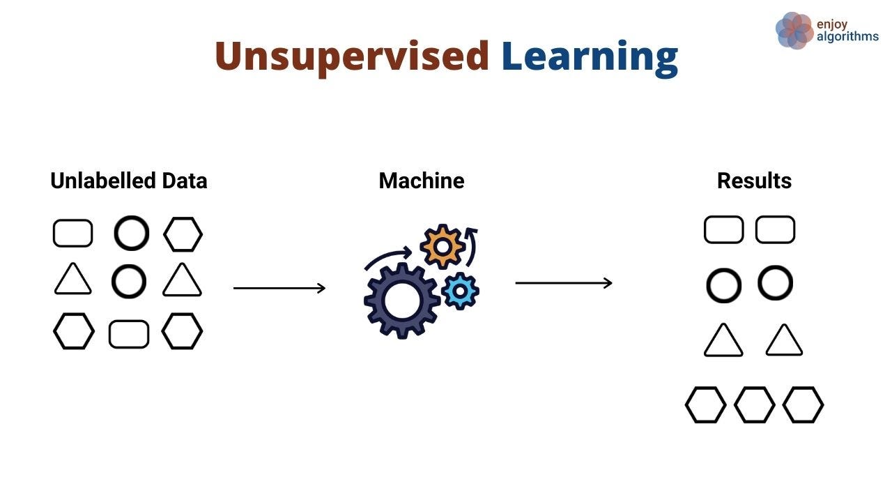
No targets anymore! The training dataset \(\mathcal D = (\boldsymbol x_i)_{i=1}^N\).

Examples of unsupervised learning tasks:

clustering
dimension reduction
discovering latent factors
searching for association rules

Clusterisation made on Iris dataset (figure 1.8 from [Murphy, 2022]):

---------------------------------------------------------------------------
ModuleNotFoundError                       Traceback (most recent call last)
Cell In[5], line 7
      5 from sklearn.mixture import GaussianMixture
      6 from sklearn.datasets import load_iris
----> 7 import seaborn as sns
      9 iris = load_iris()
     10 X = iris.data

ModuleNotFoundError: No module named 'seaborn'

Semisupervised learning#

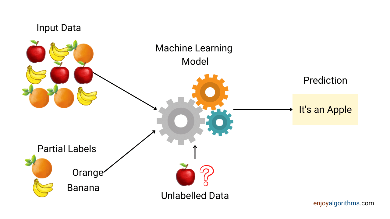
Semi-supervised learning comes into play when you have a dataset that contains both labeled and unlabeled data. Semi-supervised learning is often used in scenarios where obtaining labeled data is expensive, time-consuming, or otherwise challenging.

Reinforcement learning#

Reinforcement learning is a machine learning paradigm where an agent learns to make sequential decisions by interacting with an environment. It aims to maximize a cumulative reward signal by exploring actions and learning optimal strategies through trial and error.

TODO

Pictures from the internet is a temporary solution, try to create original ones
Add a subsection about dummy model (move something from the next chapter if necessary)
Write more about ML beyond supervised learning
Convert \(N\) and \(D\) into \(n\) and \(d\)